Getting Started
You can clone A-SLOTH to your machine with:
git clone https://gitlab.com/thartwig/asloth.git
If you encounter a problem or error at any point, you can consult the section on debugging, which contains a list of known problems and their solutions.
System Requirements and Dependencies
To run A-SLOTH you need a fortran compiler. We tested recent ifort and gfortran compilers, but you are welcone to try different ones. Set the correct compiler in the Makefile. A-SLOTH uses some features of the 2003 and 2008 standards of fortran, so very old compilers will probably not work. You will also need an Open-MP library if you want to run the code in parallel and python 3 and if you indend to use our plotting scripts. The Code is usually using a large amount of RAM. The fiducial EPS-based mode required about 4GB of RAM. We recommend 24-64 GB of RAM for modelling a full Milky Way based on the Caterpillar merger trees.
We have tested A-SLOTH and the provided tutorials on the following systems:
Ubuntu 18.04, gfortran 7.5.0 / gfortran 10.3.0 / ifort 2021.5.0, python 3.8.3
Ubuntu 20.04, gfortran 9.4.0, python 3.8.2
CentOS Linux 7, ifort 2019.2, python 3.8.9
MacOSX 10.14.6, gfortran 11.2.0 / gfortran 8.2.0, python 3.9.9 / python 3.6.13 / python 3.7.3
MacOSX 10.15.7, gfortran 9.2.0, python 3.7.10
To execute the python analysis scripts, you might need to install the additional python packages (for example with pip3 install PackageName)
numpy
scipy
matplotlib
pandas
psutil
astropy
In addition, if you want to compute a p-value for the model (comparison with observables), you need to install ‘R’ and the following python pacages.
sklearn
rpy2
Tutorials
The following tutorials will guide you through the basic functions and applications of A-SLOTH. We recommand to complete these tutorials in order. A walk-through for the tutorials is provided on YouTube.
The tutorials are based on the public release version of A-SLOTH with no other modifications. If a tutorial does not work, you might want to first reset A-SLOTH to the fiducial version, i.e., by checking git status, and by running make clean. Or you might need to first delete or rename previous output folders in the A-SLOTH directory.
If not stated otherwise, all commands should be executed from the main A-SLOTH directory.
All python scripts in these tutorials should be run with python 3.
Tutorial 1: Hello A-SLOTH
Here, we summarize how you can run A-SLOTH with fiducial settings and check your outputs with standard plotting scripts. Change to the A-SLOTH folder and compile the code with
cd asloth/
make
Then you can run A-SLOTH with the command
./asloth.exe param_template.nml
If everything goes well, you should then see the statement
  ...
 Starting main star formation and feedback loop
 Current redshift:   0.0 PROGRESS: [###############################]100.00% -- Complete
 A-SLOTH finished successfully.
Now, we can have a look at the results by running python-based plotting scripts:
python scripts/plot_asloth.py
Ideally, the script will use the newest folder to visualize the results. It will also tell you in which folder the plots are saved:
...
The directory output_DATE_TIME exists and we will use it to create plots.
Plots will be saved in output_DATE_TIME/plots/
Adopted EMP fraction in MW: 2.314815e-05
...
The resulting figures should look like this:
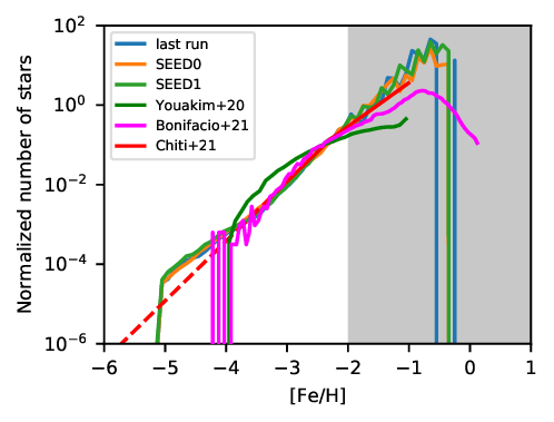
or this:
Please note: A-SLOTH is only deterministic if the same random seed, compiler, processor architecture, and optimisation flags are used. Therefore, your simulation output might look slightly different than this plot. As reference, we provide two additional reference values (SEED0, SEED1) with different random seeds to give you an idea how much the random seed can affect the results.
Tutorial 2: Vary one input parameter manually
In this tutorial, we investigate the effect of the Pop III IMF on the MDF. The fiducial model suggests Mmax=210Msun. Let’s see how observables change if we modify this fiducial value to 100Msun or 300Msun (note that the mass range of PISNe is about 140-260Msun). This tutorial consists of two steps: first, we run the 3 different models (Mmax = [100,210,300]Msun). Then we will plot the MDFs from these 3 models
Step 1: Run the three models. To run the fiducial model with Mmax=210Msun, you need to run:
make clean
make
./asloth.exe param_template.nml
Once A-SLOTH has finished, you should have one folder named output_YYYYMMDD_HHMMSS.
For better overview, you can rename this folder (not necessary, but helps later):
mv output_day_time output_Mmax210
Now, we want to run a second model with a different value for Mmax. For this purpose, we first copy the parameter file:
cp param_template.nml param_Mmax.nml
Then, we open the file param_Mmax.nml and modify the line with
IMF_max=210 ! maximum mass of PopIII IMF
to the desired value, let’s say 100, and save the parameter file. Now we can run A-SLOTH again with this new parameter file:
./asloth.exe param_Mmax.nml
This should have generated another output folder that you can rename again.
Now you can change IMF_max in param_Mmax.nml again and run A-SLOTH a third time.
At the end of this step, you should have three folders with the results of the three runs that are named
output_Mmax100
output_Mmax210
output_Mmax300
Step 2: Plot the results. Open the file scripts/plot_asloth.py and scroll to the bottom.
Change UserFolder to
UserFolder = ["output_Mmax100", "output_Mmax210", "output_Mmax300"]
and UserLabels to
UserLabels = ["Mmax=100Msun", "Mmax=210Msun", "Mmax=300Msun"]
Furthermore, set plot_newest_folder = False.
Save the file and run it with
python scripts/plot_asloth.py
The python scripts should have told you
...
Plots will be saved in output_Mmax100/plots/
...
(together with many other information).
So let’s look into this folder, which should contain the file MW_MDF.pdf, which should look like this (due to different random number generators or seeds, the figure might not look exactly like this one):
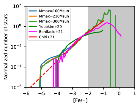
We can see that the run with Mmax=100Msun (blue) differs from the other runs in the metallicity range below [Fe/H]=-3. Congratulations! You now know how to run and compare A-SLOTH with different input parameters manually.
Tutorial 3: Explore two input parameters automatically
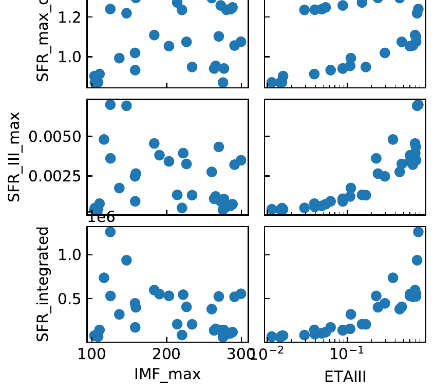
In this tutorial we want to use A-SLOTH for a parameter exploration and see which observables are most sensitive to the details of PopIII star formation. Specifically, we want to vary the upper mass limit of the PopIII IMF and the PopIII star formation efficiency. Therefore, we run many realizations and sample random pairs of these two parameters. At the end, we visualize the effect of these parameters on the observables.
Optional: you can set the variable path_output in scripts/wrapper/loop_trees.py and the variable folder_name in scripts/wrapper/analyse_trees.py to a folder in which you want to save the output. Otherwise, output will be written to your A-SLOTH folder.
The following script will run for 15-30Min:
python scripts/wrapper/loop_trees.py
This script launches a python wrapper which will run 32 x 3 EPS merger trees:
Draws random values for Mmax and ETAIII
Checks if enough RAM and CPUs are available
Launches first tree
If sufficient resources are available, it also launches a second and third EPS tree with the same input parameters, but with a different random seed.
It continues with 1)-4) until either 32 x 3 trees are completed OR until 30Min are over.
If sufficient resources are not available (RAM, CPUs, disk I/O), it will wait a few seconds and try again.
Please note: the output to terminal might seem confusing because multiple trees are running at the same time. If the python script finishes before A-SLOTH, you might not get back to the command line prompt at the end of this run. If this is the case, you can press Enter once the last tree has finished.
Once this script has finished, you should have many folders with the results in your path_output directory. In addition, the two figures RAM_histogram.pdf and CPU_histogram.pdf show you the available resources during the run. This is useful to check if any of these poses a bottleneck to the calculation.
We have prepared another script to extract, digest, and compare the data of the output folders:
python scripts/wrapper/analyse_trees.py
This script goes through all the folders, collects the input parameters from each run, calculates the observables from A-SLOTH, and eventually compares them to real observables. During the run, plots are created in the output folders. The print messages will tell you in which folders you can find the individual plots.
At the end, this script will produce the file Parameter_Exploration.dat. You can either look at this file manually, analyse it with your favourite software, or use a third script to visualize it:
python scripts/wrapper/tutorial_GridPlot.py
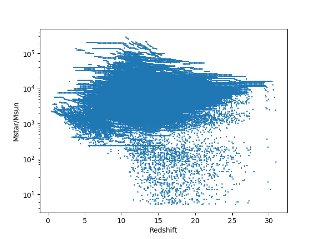
The generated figure Parameter_Exploration_tutorial.pdf should look like this cut-out:
Tutorial 4: Analyse evolution of baryons in one merger tree branch
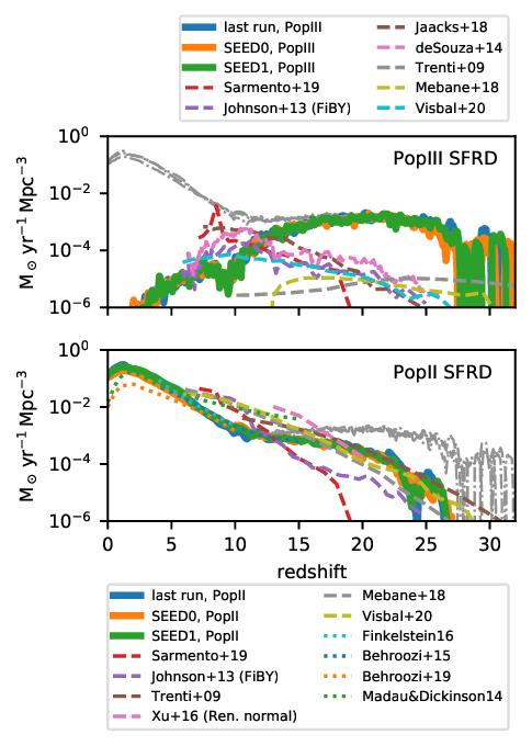
In this tutorial, we want to activate one additional compile time option in order to create a plot like this:
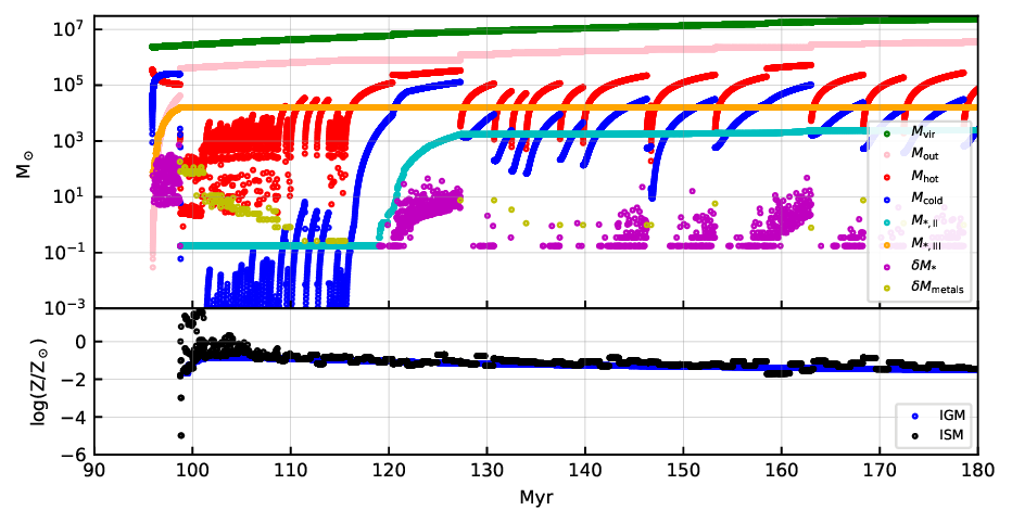 This plot shows the evolution of different baryonic quantities as function of cosmic time for one branch of the merger tree. Your plot might look slightly different depending on the random seed. For another example and explanations of the illustrated quantities, see Fig. 3 in Hartwig+22.
To generate the output for this plots, we have to activate the compiler flag OUTPUT_GAS_BRANCH. To do this, open the file src/asloth.h and activate the option by remeoving the first ! in that line.
#define OUTPUT_GAS_BRANCH
You should recompile code with
make clean
make
Then, you can run the code with
./asloth.exe param_template.nml
In your output_date_time folder you should now have the additional file t_gas_substeps.dat. To illustrate these results, you can use a python script. But first, we have to set the output folder in the script.
Open the file scripts/utilities/plot_tgas.py and in the very last line change output_folder to your output folder that was just created. Save the file and run
python scripts/utilities/plot_tgas.py
This should have generated the file t_gas.pdf in your output folder.
Tutorial 5: Output additional information from A-SLOTH
So far, we have used output files that were already implemented and written to the output folder. Now, we want to learn how users can implement their own desired output to a file.
There are various options to write to a file. One can either keep a file open and write to it incrementally during the run. Or one can write all information to a file at once at the end of the run. In this example, we will look at the subroutine write_files_reali() in the file src/to_file, which is called at the end of the run to write outputs to files.
In this file, you will find a section that starts with
!!! TUTORIAL 5: START !!!
At the moment, this code opens a file, writes a header, and closes the file. The do-loop iterates over all dark matter halos in this run and the write statement would write information for every halo. Such a file would be huge with millions of lines. Hence, it is currently deactivated by
if(.False.)then
This routine should write the redshift and stellar mass of halos. Let’s say we want this information only for PopIII-dominated halos, i.e., for halos that contain more PopIII stars than PopII stars.
Change the if-statement so that we only write information of PopIII-dominated halos to the file. Yes, you have to think how this if-statement looks like and can not simply copy it from the handbook as in previous tutorials. When you need additional information what the different node properties mean (Node%quantity), you can look in the file src/defined_types.F90 under type TreeNode.
Save the file once you have changed the if-statement. Then you can compile and run the code, as you have done in Tutorial 1. Again, you should get a new folder output_date_time.
To illustrate the results, you can open the python script scripts/utilities/tutorial5.py, set the correct output_folder, save it, and run it with
python scripts/utilities/tutorial5.py
Please note that the plot shows cumulative stellar masses, i.e., stellar masses that have formed until a certain redshift, but it does not account for stars that have already died based on their lifetime. While this plot is not immensly informative, this tutorial has shown you how to output and illustrate additional quantities from A-SLOTH. Happy coding!
Configure your simulation
The following files are relevant to change the general behaviour of the code:
Parameter file. We provide the parameter file
param_template.nml. We recommend to first create a copy of this file if you want to change these values. Numerical values in this file are calibrated to match observations, see Hartwig+22.Config file. You can find the available compile time options in the file
src/asloth.h. You have to recompile the code if you change these compiler time options.Numerical parameters. You can find additional parameters in the file
src/num_pars.F90. They are set to recommended values. You might want to change some of these parameters, such as the simulated redshift range, or the halos mass resolution.